18. June 2019
Kaggle Movie data Part 1.1
What’s going to happen?
As a first real post, I want to show a short analysis I was conducting for a job interview. So, this might be interesting for those, currently applying for a job as a data analyst. I think it is a good topic to start off this blog. Although the interview was for a company, near to the construction industry, the data set I got, again, was about movies from a kaggle page. For future posts, I try to look out for data, around building and construction.
I will split this post into different pieces. For the first part, I will closely stick to the tasks I received for the Job-Interview. Let’s get started.
Task One
The first task was simply about getting a short overview about the data. The data itself is separated into five .csv files.
|
|
Except Writer and AdditionalRating the data is referencing movie observations, even though their names imply otherwise. Because it is all about movies, the Movies data frame contains the most information. The function summary() provides the first quick overview on each variable individually.
|
|
As could have been expected, there aren’t many variables, which are purely numeric. But besides the three variables Year, imdbRating, imdbVotes I assumed something like Released, Runtime and Awards to be numeric, so lets take a quick look, at these values.
|
|
There seems to be several information inside of Awards. Specific awards are emphasized, such as Oscars, or Golden Globes. Further, there are “other” awards, which are summarised and it is always distinguished between wins and nominations. In order to have a tidy data frame, which includes all of this informations, specific variables for, e.g. Oscars, Golden Globes or Other wins and nominations should be created. Then, a more comprehensive analysis, including the awards, would be possible.
|
|
The releases appear to be in an inappropriate date format, this should easily be fixed, using the anytime-package. The character values, will become native date values.
|
|
For the runtime, there appears to be different formats, when a movie is longer 60 minutes. For further analysis, I should transform every entry, which explicitly considers hours into minutes. This should lead to one numeric variable, Runtime_min completely in minutes.
Additionally, there are some striking things to me in this summary.
- The release year ranges up to 2023, which seems a little bit high
- take a closer look at those values, where the release date is above the current date
|
|
# A tibble: 38 x 3
   Title                                                  imdbID     Year
   <chr>                                                  <chr>     <dbl>
 1 Inside Me                                              tt6195774  2023
 2 The Zero Century: Harlock                              tt7110972  2023
 3 Austin Powers Meets Monty Python Meets the Whole World tt4977768  2022
 4 Grace AKA Bubbie                                       tt5891084  2022
 5 Fast & Furious 10                                      tt5433140  2021
 6 The Silver Unknown                                     tt5235900  2021
 7 Power Hungry Animals 3                                 tt6521788  2021
 8 Star Trek 5                                            tt4756234  2021
 9 Spooky Jack                                            tt7208370  2021
10 The Boss Baby 2                                        tt6932874  2021
When opening the corresponding imdb page of the first three entries, we can observe some peculiarities of the data. The first Movie doesn’t have a current release date and a new original title. The second movie, also doesn’t have a release date and the third movie doesn’t even exist. All in all, it doesn’t promote the quality of the date and I would exclude unreleased movies from the data.
Votes & Ratings
As observable above, there is a huge number of NA's among imdbRating and imdbVotes. I’m not sure, whether it is due to the data’s quality or if really only a smaller part of all movies are rated at all. I should take a look at non-rated movies and check with the real entries on imdb.com. For now, this appears as too much work for me. Maybe later, I will take a closer look. But for now, I will look closer at the distribution and correlation of rating and votes.
For this, I want only observation, which have been voted on. Based on the imdb rules, only movies can get a mean rating, if there are more than 25.000 votes. So lets filter the data for these requirements.
|
|
A simple correlation scatter plot should reveal a possible connection between these two features. But based on the large number of votes for the top movie, I assume several outliers. I don’t want to look for them in the data separately but I’d like to see them right in the plot. The function geom_tex() from ggplot2 can put their labels next to the points. But I only want the outliers to be displayed, so I define further restrictions. Number of votes has to be above 1.500.000 and the mean rating should be higher 9.0
|
|
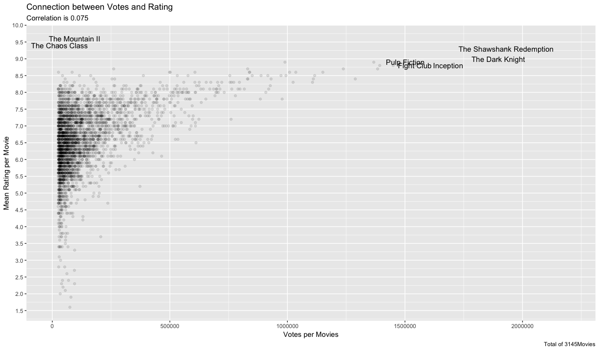
The correlation between votes and rating is very small, but some kind of pattern is evolving nevertheless. Movies with a very low rating (below 5.0) don’t cross the 250.000 votes mark and are generally quite low. The contrary for a high number of votes. Above 500.000 votes, the min rating is at around 6.5 Above 1.000.000, the worst rating is at around 8.25. I would interpret this with a feedback loop. If a movie has a low rating, less people care about/watch the movie and hence rate it on imdb. But if a movie already has a high rating, it is marked as a good movie, more people are attracted to watch it and give it a good rating. Based on this data, a movie can only have a high number of votes, if it has a high rating. Focused shitstorms, like on could assume with cpt. Marvel, i.e. high number of votes and a very low rating, can’t be observed.
Next to the great movies, with many votes we can also see another group, which has a good rating, but doesn’t get that many votes. I would consider The Mountain II and The Chaos Class as hidden gems. How does this fit into my feedback loop theory. There are two movies, with an outstanding rating, shouldn’t they get much more attention/votes? Here’s the thing, both movies are not listed in the top 250 charts, despite their unmatched rating. I don’t know why, maybe both movies miss some properties needed for the top list. Maybe it is a conspiracy to promote American movies ;). But i think, this is a very interesting point and should be further investigated, maybe by doing some web scraping on the imdb-database myself.
Most often occurred writers
Finally, I wanted to take a look at the writer file and see, which writers are credited the most. This is very straight forward. The only problem is, that several writers have multiple credits per movie. So I have to create a data frame with distinct combinations of writer and movie and then group by individual writers. The results can be plotted afterwards.
|
|
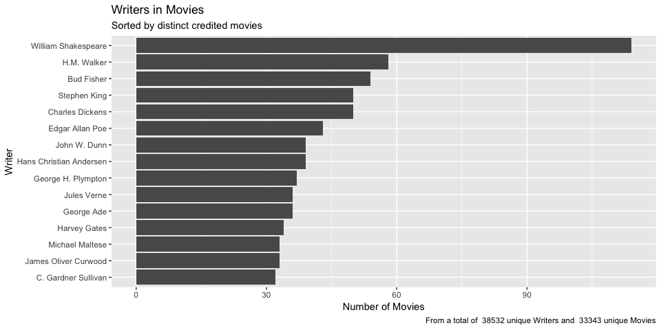
From a quick look, the most writer aren’t explicit writer of movie screenplay but traditional book authors. So in this dataset the most writers are credited based on their back catalogue and corresponding movie adaptations. I should validate this, by looking into some movie writers. Maybe I can find a way to filter some thing like original screenplay.
This is it, for the first task, I got for my latest job application. The task sheet contained two additional tasks, which I will show in my next post. This will be about finding the director, directing the most movies and my first touches of network analyses.